Generator Network
Now that we have understood the theory behind Cycle GANs, it is time for us to look at the implementation. In this article, we will have a look at the Generator architecture used in the cycle consistent image to image translation article.
NOTE : Please refer to our previous blogs to get a theoretical understanding behind cycle consistent networks.
In the implementation section of this paper, the authors state that the Generator architecture used, was obtained from the paper titled Perceptual Losses for Real Time Style Transfer by Justin Johnson et. al.
Justin Johnson et. al. utilize perceptual losses to perform style transforms between two set of images. They also perform single image super resolution. They claim that their implementation provides similar results when compared to optimization models while being three orders in magnitude faster. Now that’s an amazing feat!
They state that their architecture does not rely only on pixel losses but also on perceptual losses which is the most important as small translations and rotations of the image give large pixel losses which is not the case when considering perceptual losses. This results in absolutely stunning outputs as shown in their paper.
However, we shall not get into the perceptual losses and their benefits in this article as that is not our major goal. Our motive to understand their architecture is limited to their Generator architecture which generates the amazing outputs and also does this at a really fast pace.
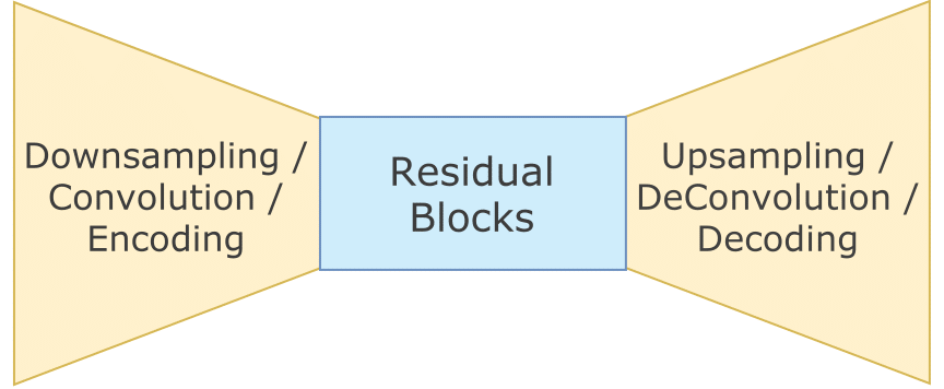
The Generator used in this implementation involves three parts to it:
In-network Downsampling, Several Residual Blocks and In-network Upsampling
In-Network Downsampling
This part of the Generator consists of two Convolution Networks, each followed by Spatial Batch Normalization and a ReLu activation function. Each convolution network uses a stride of 2 so that downsampling can occur. The first layer has a kernel size of 9x9 while the second layer has a kernel size of 3x3.
Residual Blocks
The concept of Residual Blocks was introduced by Kaiming He et. al. in their paper titled Deep Residual Learning for Image Recognition. Each Residual Block consists of two Convolution Layers. The first Convolution Layer is followed by Batch Normalization and ReLu activation. The output is then passed through a second Convolution Layer followed by Batch Normalization. The output obtained from this is then added to the original input.
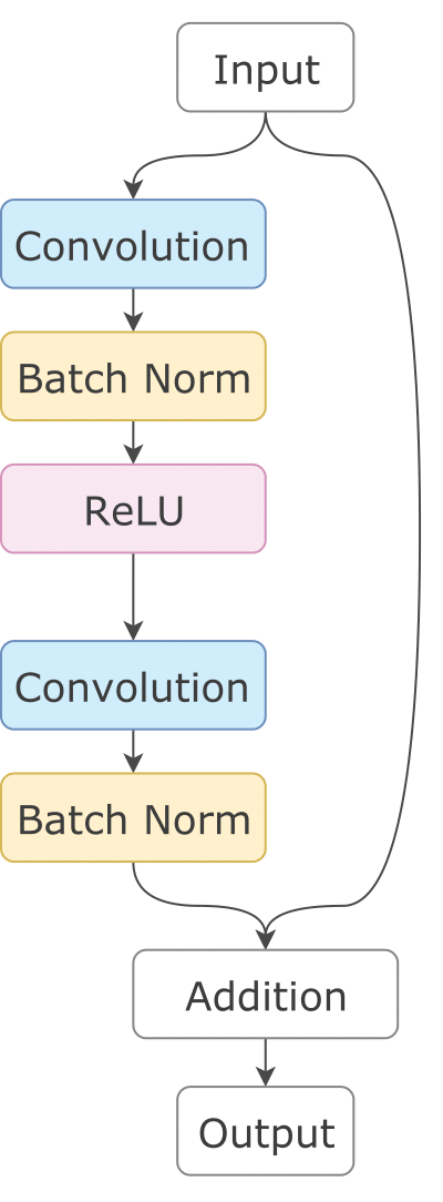
To understand this in more depth, you can look at this blog where the above image was taken from. Each convolution layer in residual blocks has a 3x3 filter. The number of Residual Blocks depens on the size of the input image. For 128x128 images, 6 residual blocks are used and for 256x256 and higher dimensional images, 9 residual blocks are used.
In-network Upsampling
This part consists of two convolution layers. They are fractionally strided with a stride value of $\frac{1}{2}$ . The first convolution layer has a kernel size of 9x9 while the last layer has a kernel size of 9x9. The first layer is followed by Batch Normalization and ReLU activation while the second convolution layer is followed by a Scaled Tanh function so that the values can fall between [0,255] as this layer is the output layer.
The entire Feedforward Generator Network starts off with Downsampling, followed by Residual Blocks and ends with Upsampling.
The benefits of using such a network is that it is computationally less expensive compared to the naive implementation and provides large effective receptive fields that lead to high quality style transfers in the output images.
Implementation:
Our implementation of the Generator can be found here
Network Layout
Following is the description of the overall generator network layer by layer configuration. This is the exact model that we have implemented in our generator code.
| Layer Number | Layer | Kernel | Stride | Dimension I/O | Channels I/O |
|---|---|---|---|---|---|
| 1 | Conv2d | 7 | 1 | 256—256 | 3—64 |
| 2 | BatchNorm2d | - | - | 256—256 | 64—64 |
| 3 | ReLU | - | - | 256—256 | 64—64 |
| 4 | Conv2d | 3 | 2 | 256—128 | 64—128 |
| 5 | BatchNorm2d | - | - | 128—128 | 128—128 |
| 6 | ReLU | - | - | 128—128 | 128—128 |
| 7 | Conv2d | 3 | 2 | 128—64 | 128—256 |
| 8 | BatchNorm2d | - | - | 64—64 | 256—256 |
| 9 | ReLU | - | - | 64—64 | 256—256 |
| 10 | Conv2d | 3 | 1 | 64—64 | 256—256 |
| 11 | BatchNorm2d | - | - | 64—64 | 256—256 |
| 12 | ReLU | - | - | 64—64 | 256—256 |
| 13 | Convd2d | 3 | 1 | 64—64 | 256—256 |
| 14 | BatchNorm2d | - | - | 64—64 | 256—256 |
| 15 | 9+14 | - | - | 64—64 | 256—256 |
| 16 | Conv2d | 3 | 1/2 | 64—128 | 256—128 |
| 17 | BatchNorm2d | - | - | 128—128 | 128—128 |
| 18 | ReLU | - | - | 128—128 | 128—128 |
| 19 | Conv2d | 3 | 1/2 | 128—256 | 128—64 |
| 20 | BatchNorm2d | - | - | 256—256 | 64—64 |
| 21 | ReLU | - | - | 256—256 | 64—64 |
| 22 | Conv2d | 7 | 1 | 256—256 | 64—3 |
| 23 | TanH | - | - | 256—256 | 3—3 |
Repeat steps 10 to 15 nine times to have 9 residual blocks
Code Snippet
A code snippet for our simplified discriminator is shown below. The generator function have 4 high level operations : Batch Normalization, Convolution, De-Convolution and Residual Block . Lets follow the same order and write the generator network.
Batch Normalization
This function is relatively straightforward. Given a set of Logits we have to normalize them according to $BN(x_i) = \gamma(\frac{x_i - \mu_B}{\sqrt{\sigma^2_B + \epsilon}}) + \beta$. We will add small float added to variance to avoid dividing by zero.
# Function for Batch Normalization
def batchnorm(Ylogits):
    bn = tf.contrib.layers.batch_norm(Ylogits, scale=True, decay=0.9, epsilon=1e-5, updates_collections=None)
    return bn
Convolution & De-Convolution
# Function for Convolution Layer
def convolution_layer(input_images, filter_size, stride, o_c=64, padding="VALID", scope_name="convolution"):
    with tf.variable_scope(scope_name):
        conv = tf.contrib.layers.conv2d(input_images, o_c, filter_size, stride, padding=padding, activation_fn=None,
                                        weights_initializer=tf.truncated_normal_initializer(stddev=0.02))
        return conv
# Function for deconvolution layer
def deconvolution_layer(input_images, o_c, filter_size, stride, padding="VALID", scope_name="deconvolution"):
    with tf.variable_scope(scope_name):
        deconv = tf.contrib.layers.conv2d_transpose(input_images, o_c, filter_size, stride, activation_fn=None,
                                                    weights_initializer=tf.truncated_normal_initializer(stddev=0.02))
        return deconv
Residual Block
# Function for Residual Block
def residual_block(Y, scope_name="residual_block"):
    with tf.variable_scope(scope_name):
        Y_in = tf.pad(Y, [[0, 0], [1, 1], [1, 1], [0, 0]], "REFLECT")
        Y_res1 = tf.nn.relu(batchnorm(convolution_layer(Y_in, filter_size=3, stride=1, o_c=output_channels * 4, scope_name="C1")))
        Y_res1 = tf.pad(Y_res1, [[0, 0], [1, 1], [1, 1], [0, 0]], "REFLECT")
        Y_res2 = batchnorm(convolution_layer(Y_res1, filter_size=3, stride=1, padding="VALID", o_c=output_channels * 4, scope_name="C2"))

        return Y_res2 + Y
Network’s Brain
with tf.variable_scope(scope, reuse=tf.AUTO_REUSE):

    # Need to pad the images first to get same sized image after first convolution
    input_imgs = tf.pad(input_imgs, [[0, 0], [3, 3], [3, 3], [0, 0]], "REFLECT")

    YD0 = tf.nn.relu(batchnorm(convolution_layer(input_imgs, filter_size=7, stride=1, o_c=output_channels, scope_name="D1")))
    YD1 = tf.nn.relu(batchnorm(convolution_layer(YD0, filter_size=3, stride=2, o_c=output_channels * 2, padding="SAME", scope_name="D2")))
    YD2 = tf.nn.relu(batchnorm(convolution_layer(YD1, filter_size=3, stride=2, o_c=output_channels * 4, padding="SAME", scope_name="D3")))

    # For Residual Blocks
    for i in range(1, no_of_residual_blocks + 1):
        Y_res = residual_block(YD2, scope_name="R" + str(i))

   # For Upsampling
   YU1 = tf.nn.relu(batchnorm(deconvolution_layer(Y_res, output_channels * 2, filter_size=3, stride=2, padding="SAME", scope_name="U1")))
   YU2 = tf.nn.relu(batchnorm(deconvolution_layer(YU1, output_channels, filter_size=3, stride=2, padding="SAME", scope_name="U2")))
   Y_out = tf.nn.tanh(convolution_layer(YU2, filter_size=7, stride=1, o_c=3, padding="SAME", scope_name="U3"))

   return Y_out
With this we are done with the proper implementation of the generator network.
Feel free to reuse our Generator code, and of course keep an eye on our blog. Comments, corrections and feedback are welcome.
Sources
- Unpaired Image-to-Image Translation using Cycle-Consistent Adversarial Networks
- Image-to-Image Translation with Conditional Adversarial Networks
- Training and investigating Residual Nets
- Perceptual Losses for Real-Time Style Transfer and Super-Resolution