
Minimal Convolutional Neural Network
Before diving into complex neural world of generative adversarial nets, probably its a good idea to start with a simple convolutional neural network. We will walk through a minimal implementation of CNN with standard MNIST dataset.
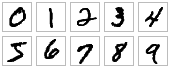
The MNIST dataset comprises 60,000 training examples and 10,000 test examples of the handwritten digits 0–9, formatted as 28x28-pixel monochrome images.
Flash Back : How CNN works?
As we have discussed in previous post, convolutional neural networks (CNNs) are the current state-of-the-art model architecture for image classification tasks. CNNs apply a series of filters to the raw pixel data of an image to extract and learn higher-level features, which the model can then use for classification. CNNs contains three components:
-
Convolutional layers, which apply a specified number of convolution filters to the image.
-
Pooling layers, which is an operation of shrinking the image while preserving the most common information in them.
-
Dense (fully connected) layers, which takes the high-level filtered images and translate them into votes.
Note: For a more comprehensive walk through of CNN architecture, see Stanford University’s Convolutional Neural Networks for Visual Recognition course materials.
Tensor flow skeleton
We will follow official guide from TensorFlow to create our skeleton code for CNN implementation:
from __future__ import absolute_import
from __future__ import division
from __future__ import print_function
# Imports
import numpy as np
import tensorflow as tf

tf.logging.set_verbosity(tf.logging.INFO)

# Our application logic will be added here

if __name__ ==  "__main__": tf.app.run()
The complete, final code can be found here.
Classifier Architecture
The high level pipeline for our CNN Classifier is :
| Layer | Shape | Activation |
|---|---|---|
| input | Batch, 28, 28, 1 | NA |
| Convolution | Applies 32 5x5 filters | ReLU |
| Pooling | Performs max pooling, 2x2 filter & stride, 2 | NA |
| Convolution | Applies 64 5x5 filters | ReLU |
| Pooling | Again, Performs max pooling, 2x2 filter & stride, 2 | NA |
| Dense | 1,024 neurons | dropout rate 0.4 |
| Logit | 10 neurons | one for each digit target class (0–9) |
If you carefully note, our last logits layer will give a 10 node output. We can derive probabilities from our logits layer by applying softmax activation. We compile our predictions in a dictionary, and return an EstimatorSpec object. For both training and evaluation, we need to define a loss function that measures how closely the model’s predictions match the target classes. For multi-class classification problems like MNIST, cross entropy is typically used as the loss metric.
we defined loss for our CNN as the softmax cross-entropy of the logits layer and our labels. Let’s configure our model to optimize this loss value during training. We’ll use a learning rate of 0.001 and stochastic gradient descent as the optimization algorithm. In addition, to add accuracy metric in our model, we define eval_metric_ops dictionary in EVAL mode.
Code
def cnn_model_fn(features, labels, mode):
  """Model function for CNN."""
  # Input Layer
  input_layer = tf.reshape(features["x"], [-1, 28, 28, 1])

  # Convolutional Layer #1
  conv1 = tf.layers.conv2d(
      inputs=input_layer,
      filters=32,
      kernel_size=[5, 5],
      padding="same",
      activation=tf.nn.relu)

  # Pooling Layer #1
  pool1 = tf.layers.max_pooling2d(inputs=conv1, pool_size=[2, 2], strides=2)

  # Convolutional Layer #2 and Pooling Layer #2
  conv2 = tf.layers.conv2d(
      inputs=pool1,
      filters=64,
      kernel_size=[5, 5],
      padding="same",
      activation=tf.nn.relu)
  pool2 = tf.layers.max_pooling2d(inputs=conv2, pool_size=[2, 2], strides=2)

  # Dense Layer
  pool2_flat = tf.reshape(pool2, [-1, 7 * 7 * 64])
  dense = tf.layers.dense(inputs=pool2_flat, units=1024, activation=tf.nn.relu)
  dropout = tf.layers.dropout(
      inputs=dense, rate=0.4, training=mode == tf.estimator.ModeKeys.TRAIN)

  # Logits Layer
  logits = tf.layers.dense(inputs=dropout, units=10)

  predictions = {
      # Generate predictions (for PREDICT and EVAL mode)
      "classes": tf.argmax(input=logits, axis=1),
      # Add `softmax_tensor` to the graph. It is used for PREDICT and by the
      # `logging_hook`.
      "probabilities": tf.nn.softmax(logits, name="softmax_tensor")
  }

  if mode == tf.estimator.ModeKeys.PREDICT:
    return tf.estimator.EstimatorSpec(mode=mode, predictions=predictions)

  # Calculate Loss (for both TRAIN and EVAL modes)
  loss = tf.losses.sparse_softmax_cross_entropy(labels=labels, logits=logits)

  # Configure the Training Op (for TRAIN mode)
  if mode == tf.estimator.ModeKeys.TRAIN:
    optimizer = tf.train.GradientDescentOptimizer(learning_rate=0.001)
    train_op = optimizer.minimize(
        loss=loss,
        global_step=tf.train.get_global_step())
    return tf.estimator.EstimatorSpec(mode=mode, loss=loss, train_op=train_op)

  # Add evaluation metrics (for EVAL mode)
  eval_metric_ops = {
      "accuracy": tf.metrics.accuracy(
          labels=labels, predictions=predictions["classes"])}
  return tf.estimator.EstimatorSpec(
      mode=mode, loss=loss, eval_metric_ops=eval_metric_ops)
Recommendation: Please visit TensorFlow
Getting Startedguide for specifics of the above layers.
CNN predicting MNIST
The code is quite naive to implement on any decent machine with a CPU. Depending on your CPU’s performance, the runtime is decided.
Here’s the snapshot of the final result :
INFO:tensorflow:loss = 2.36026, step = 1
INFO:tensorflow:probabilities = [[ 0.07722801  0.08618255  0.09256398, ...]]
...
INFO:tensorflow:loss = 2.13119, step = 101
INFO:tensorflow:global_step/sec: 5.44132
...
INFO:tensorflow:Loss for final step: 0.553216.

INFO:tensorflow:Restored model from /tmp/mnist_convnet_model
INFO:tensorflow:Eval steps [0,inf) for training step 20000.
INFO:tensorflow:Input iterator is exhausted.
INFO:tensorflow:Saving evaluation summary for step 20000: accuracy = 0.9733, loss = 0.0902271
{'loss': 0.090227105, 'global_step': 20000, 'accuracy': 0.97329998}
Here, we’ve achieved an accuracy of 97.3% on our test data set.
Future Implementations
One of the eye catching implementation is done by Jon Bruner and Adit Deshpande form the O’Reilly interactive tutorial on generative adversarial networks.

In this implementation, they have managed to produce MNIST dataset itself from the Gaussian Noise using DCGANS.
Feel free to reuse our CNN code, and of course keep an eye on our blog. Comments, corrections and feedback are welcome.